

Introduction
Scaling up machine learning models – in terms of model size, dataset size, and compute – has led to dramatic improvements in performance on language and vision tasks. In recent years, researchers have observed striking neural scaling laws: empirical relationships showing that as we increase these factors, the model’s error (or loss) follows a predictable decline (often a power-law). In other words, bigger models trained on more data with more compute tend to get predictably better. This blog post provides an overview of neural scaling laws, focusing on what has been learned from language models and how those insights compare to vision models. We’ll summarize key findings from Kaplan et al. (2020) on “Scaling Laws for Neural Language Models”, discuss theoretical interpretations, examine similarities and differences in scaling for vision, and consider practical implications for model design and training. Along the way, we’ll highlight important charts and what they show. We’ll also discuss where these empirical laws might break down – such as the emergence of unexpected capabilities or hitting fundamental data limits – and reflect on what this means for the future of large “foundation” models in AI.
Sample Efficiency and Overfitting Trends
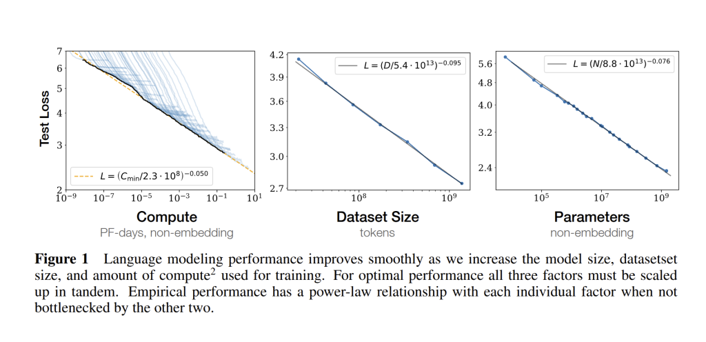
Before diving into sample efficiency and overfitting, it helps to see the big picture. Kaplan et al. (2020) showed that language modeling loss scales in a remarkably simple way with three factors: the number of non-embedding parameters N (model size), the dataset size in tokens D, and the training compute C (roughly proportional to FLOPs used). Figure 1 from their paper illustrates these relationships: in each case, test loss falls along a straight line on a log-log plot, indicating a power-law dependence that holds over 6 to 7 orders of magnitude.
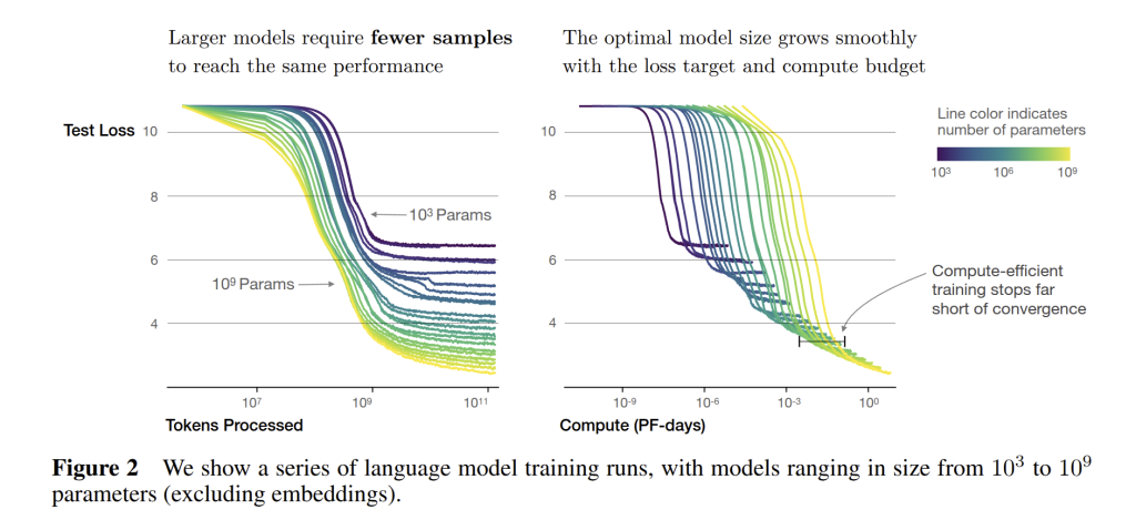
One interesting consequence of these scaling laws is the notion that larger models are more sample-efficient. Empirically, a 10× bigger model might achieve the same loss as a smaller model with only a fraction of the training data or steps. This was observed in the smooth horizontal shifts of learning curves (see Fig. 2 below): bigger models essentially learn faster. Why might that be? Intuitively, a more expressive model can absorb the training data’s patterns more readily and it has enough parameters to quickly fit the dominant trends in the data and then continue improving on subtler patterns. In contrast, a small model struggles to even represent the complex structure, so it needs to see many more examples to lower its loss. In practical terms, this means if you can afford a larger model, you save data and training time to reach a target performance. This is one reason large models like GPT-3, GPT-4, etc. achieve good results even on relatively limited fine-tuning datasets – the pre-trained large model can make the most of the small fine-tuning set.
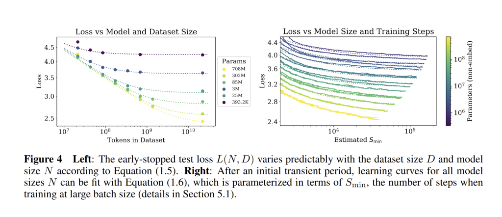
Kaplan et al. formalized overfitting in a neat way: they found the extent of overfitting depends predominantly on the ratio of model size to dataset size. If you hold dataset size fixed and keep increasing model parameters, you eventually get diminishing returns (the loss approaches an asymptote given by the finite data). Conversely, for a fixed model, increasing data has diminishing returns once the model capacity is fully utilized. They encapsulated this in the combined formula for
L(N,D) = \left(\frac{N_c}{N}\right)^{\alpha_N} + \left(\frac{D_c}{D}\right)^{\alpha_D} (see Fig. 4 below).
A practical rule-of-thumb that emerged: when you increase model size by a factor of 8, you should have roughly 5× more data to keep the model learning instead of overfitting (see Fig. 9 below). In other words, data needs to grow sublinearly with parameters. This sublinear growth (exponent ~0.74) implies that larger models require less additional data per new parameter than smaller models did to maintain the same generalization gap. This reflects the fact that many of the easier patterns in the data can be learned with a modest amount of data, and a bigger model can capture those quickly; adding more parameters yields diminishing returns unless more data is added to uncover finer-grained patterns, but the data requirement grows slower than model size.
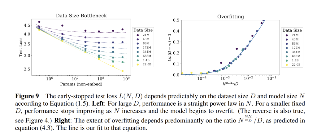
This trend held in the studied range, and no sudden overfitting cliff was observed – just smooth diminishing returns. Of course, if one naively scales model size without adding data or regularization, overfitting will eventually occur. But in practice, with early stopping or limited training as prescribed by compute-optimal scaling, large models were observed to generalize very well. Scaling laws thus provide a quantitative handle on when overfitting occurs: primarily when \frac{N^{\alpha_N}}{D} grows too large. This helps in planning how much data is needed as model size increases to stay in the healthy regime.
Compute-Optimal Training Regimes
Another major takeaway from Kaplan et al. is how to think about distributing a fixed compute budget. Traditionally, if you had, for example, 10^{20} FLOPs to spend on training, you might pick a model size arbitrarily and train it until you ran out of compute. Scaling law analysis instead lets us optimize that choice.
The idea of compute-optimal model size means: for a given total compute C, there is an ideal pair of (N, number of training steps) that minimizes final loss. Too small a model – you do not fully utilize the compute because even if you train to convergence it will not reach as low a loss as a larger model could. Too large a model – you under-train it given the compute, stopping too early before it reaches its potential.
Kaplan et al. derived that the optimal model size grows rapidly with compute: N_{\text{opt}} \propto C^{0.73} (see Fig. 14 below), so a 10× increase in compute should make the model about 5× larger.
Meanwhile, the optimal number of training steps grows very slowly: S_{\text{opt}} \propto C^{0.03} (see Fig. 14 below)
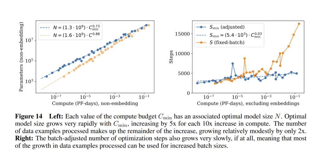
In practical terms, most of your extra compute should go into a bigger model, not into longer training. They summarized this as: as we scale up, we should predominantly increase model size NNN, while simultaneously scaling up batch size, with negligible increase in the number of serial steps. This strategy of a big model with relatively few training steps (perhaps even less than one epoch), yields the lowest loss for the compute spent.
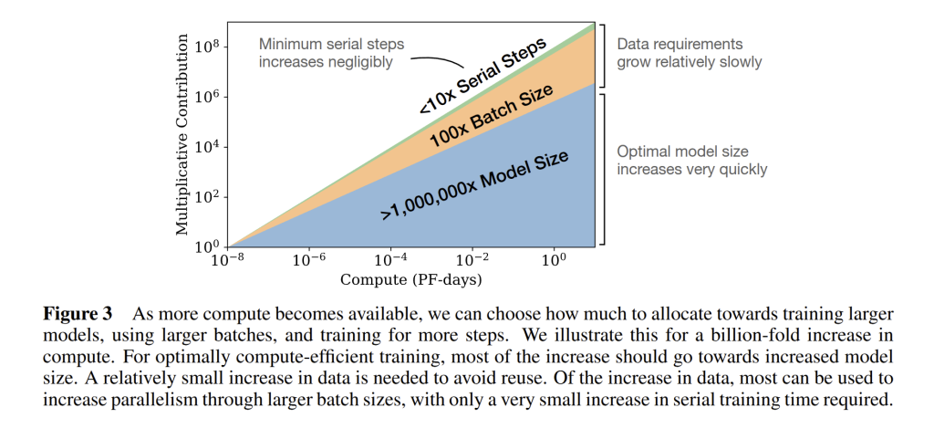
To illustrate, they gave a concrete example: suppose you suddenly had 1,000,000× more compute (see Fig. 3 below). Their scaling laws predict you would make your model approximately 10^4 x larger in parameters, use about 10^3 × more data (still only training for a small number of epochs), and increase batch size massively to use that data efficiently in parallel. You would not train for a million times more iterations – that would be wasteful and cause overfitting.
This was a shift in how large-scale training is viewed. Later, in 2022, DeepMind’s Chinchilla results refined these numbers, showing that many existing models were not trained in a compute-optimal way – notably GPT-3 (175B parameters, ~300B tokens) was under-trained for its size, meaning it should have been either smaller or trained on more data for the given compute. This refinement changed how practitioners plan large-scale model training.
Scaling Laws in Vision Models: Parallels and Contrasts
In the vision domain, scaling behaviors largely mirror those found in language models, although there are domain-specific nuances. Research over the past few years has shown that tasks like image classification and generative image modeling exhibit similar power-law relationships between performance and scale.
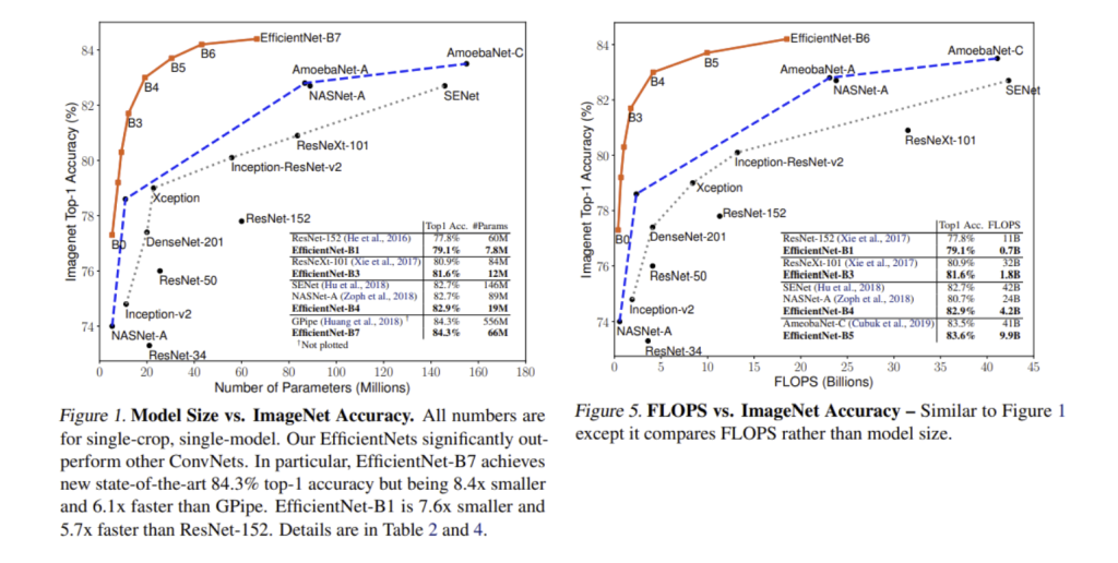
For example, the EfficientNet family of convolutional neural networks was scaled up using a compound scaling strategy and achieved accuracy improvements on ImageNet that followed an approximate power-law with respect to model size (see Fig. 1 & 5 below). This is analogous to language models, where error decreases roughly linearly in log-log space with increased model parameters, dataset size, or compute.
However, some vision tasks encounter limits sooner. Many supervised vision datasets have intrinsic label noise or ambiguity, which sets a lower bound on achievable error. As models approach this Bayes error rate, scaling curves can bend or flatten earlier than in language modeling, where the entropy limit has not yet been reached. For instance, once human-level performance is approached in classification, further scale yields diminishing returns unless more data or higher-quality labels are introduced.
In generative vision models, such as unsupervised image modeling, scaling laws appear more robust. Work extending Kaplan et al.’s analysis to image, video, and audio modeling found consistent power-law trends, suggesting that when effectively unlimited data is available, vision models benefit from scale in a similar way to text models.
Just as in language models, the shape of the network (depth vs width) plays a secondary role compared to total parameter count. Vision models, however, have historically optimized scaling along several axes, including input resolution. EfficientNet’s compound scaling, for instance, adjusts depth, width, and resolution according to fixed exponents to maximize performance for a given compute budget. In Transformer-based vision models such as ViT, scaling up parameters with sufficient training data produces smooth improvements in performance, closely resembling the trends seen in NLP.
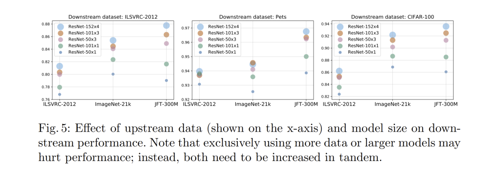
Empirical results from models like CLIP, which trained on hundreds of millions of image–text pairs, show that zero-shot accuracy improves predictably with log(model size) and log(data size), without clear saturation before data exhaustion. Similarly, the Big Transfer (BiT) project demonstrated that pretrained accuracy on ImageNet scales with dataset size across several orders of magnitude, and larger architectures benefit more from larger datasets (see Fig. 5 below).
One practical difference is that vision research often places more emphasis on compute-efficient architecture design due to deployment constraints. Studies have produced scaling laws that relate architectural hyperparameters to optimal performance per FLOP, allowing practitioners to match the accuracy of larger models with smaller, better-shaped ones. While this type of architectural optimization is less common in NLP scaling, it plays a more important role in vision because inference cost per parameter can vary widely depending on design choices.
Overall, vision and language models share the same fundamental scaling behavior: increasing model size and data leads to predictable, diminishing-returns improvements in performance. The constants and exponents may differ between domains due to differences in data complexity, availability, and task noise, but the underlying principle that scale yields gains remains consistent.
Theoretical Perspectives on Scaling Laws
Several theoretical ideas have been proposed to explain why neural networks exhibit such clean power-law scaling of error or loss with respect to model size and dataset size. While a complete theory is still under development, the main perspectives are as follows.
One approach relates the observed exponents to the effective dimensionality of the data or the target function. If the data distribution has intrinsic dimension d, classical approximation theory suggests that to reduce error you must resolve increasingly finer details in that d-dimensional manifold. In simple interpolation arguments, the typical spacing between points in the dataset scales as D^{-1/d} when you have D samples. For smooth target functions, the interpolation error might scale like the square of that spacing, giving \text{error} \sim D^{-2/d}. In an idealized piecewise-linear model with L2 loss, one could imagine even steeper scalings like D^{-4/d}. If d is large, the exponent \alpha in L(D) \propto D^{-\alpha} will be small, as observed in practice for large-scale language models.
Bahri et al. distinguish two regimes. In the variance-limited regime, model capacity is effectively infinite and performance is limited by sampling noise; error scales with sample size due to variance reduction, often like 1/D or similar. In the resolution-limited regime, performance is limited by the finiteness of model capacity and data coverage, leading to a power law L(N) \propto N^{-\alpha_N} or L(D) \propto D^{-\alpha_D}. Empirically, modern large neural networks tend to operate in the resolution-limited regime, where scaling up parameters or data directly improves the “resolution” of the learned function.
Another perspective treats a complex task such as language modeling as a collection of many subtasks with varying difficulty. If the distribution of these subtasks’ difficulty or irreducible error follows a power law, then as model size increases it progressively solves more of them, starting with the easiest. Integrating over such a heavy-tailed distribution yields an overall power-law improvement in aggregate loss. This could also explain why models seem to learn “broad strokes” first and then increasingly rare, fine-grained patterns.
Some researchers propose that scaling laws arise from general statistical properties of natural data distributions, such as fractal-like structure or Zipf’s law in language. In this view, the exact micro-level mechanism in the network is less important; the power-law exponents are determined primarily by the statistics of the task. Different domains (text, images) may belong to different “universality classes” with different exponents, but the overall form L \sim k X^{-\alpha} remains.
Although none of these perspectives fully derive the observed constants like \alpha_N \approx 0.076 in language models, they provide plausible frameworks connecting data complexity, task structure, and optimization to the emergence of smooth empirical scaling laws.
When Might the Scaling Laws Break?
With all the enthusiasm about scaling, it is important to ask: will these trends hold forever? The short answer is likely no – at some point, every exponential trend meets a wall or a regime change. Several potential breakpoints have been discussed by researchers.
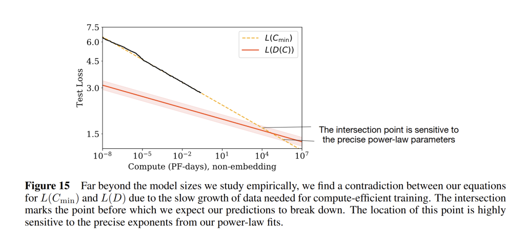
Kaplan et al. noted that eventually the power-law scaling must slow down or stop as we approach the fundamental entropy of the data distribution. For language modeling, no matter how large the model, one cannot get below the irreducible uncertainty in predicting the next token. As loss approaches that asymptote, the gains will taper off. In their extrapolations, they found a contradiction at very large scales: beyond about 10^{12} parameters and 10^{12} tokens, the predicted compute-optimal loss would dip below what the data scaling law would allow (see Fig. 15 below). This suggests that before reaching that point, at least one assumption must break. In practice, the most immediate limit is data – we may run out of high-quality training text well before these scales. The Chinchilla analysis (Hoffmann et al., 2022) refined the scaling laws to emphasize a higher optimal data-to-parameter ratio, showing that models like GPT-3 were under-trained given their size.
Another way scaling might break is through unexpected jumps in capability. Certain skills in language models do not improve smoothly but seem to appear suddenly when model size passes a threshold. Examples include arithmetic, multi-step reasoning, or few-shot learning. Below that scale, performance may be near random, then it leaps upward. While average loss may still follow a smooth power-law, specific abilities can exhibit non-linear scaling, suggesting phase-transition-like behavior in learned representations.
Additionally, the current scaling laws apply to a given family of architectures and training objectives. If a better architecture or method appears that achieves lower loss with fewer parameters, the previous scaling law would no longer apply. Retrieval-augmented models, better data curation, or different objectives could bend the curve in a favorable way, effectively giving a new scaling regime with better exponents.
Furthermore, even if scaling laws continue mathematically, practical constraints may stop us from following them. Training extremely large models could be infeasible due to hardware, energy, or cost limitations. Because the exponents are small, each additional point of improvement may require a huge increase in compute. At some point, this becomes uneconomical, shifting focus toward efficiency improvements rather than pure scale.
Conclusion: The Future of Foundation Models and Scaling
The trajectory of foundation models will likely involve scaling along less obvious dimensions than raw parameter count or token volume. Advances may come from integrating richer modalities, structuring models for lifelong learning, and leveraging interactive feedback loops with users or environments. Training objectives might evolve to include reasoning traces, tool use, or grounding in physical or simulated contexts, which could open new scaling axes orthogonal to N, D, and C.
Infrastructural innovation will be essential to sustain meaningful progress. This could mean hardware designed to support extremely high-bandwidth interconnects, adaptive parallelism strategies that minimize idle compute, or distributed storage systems optimized for streaming massive, diverse datasets. Such improvements could shift the effective cost curve, making previously prohibitive scales practical.
The evaluation of model progress will also need to mature. Beyond aggregate loss, the community may standardize richer benchmarks that track compositional reasoning, long-horizon planning, or real-time adaptation. These metrics will help determine whether new scaling directions translate to usable gains in capability and robustness.
Finally, the interplay between algorithmic efficiency and scale will become more critical. Research into architectures that offer sublinear growth in compute per performance gain may redefine what is considered optimal scaling. In this next phase, the focus could shift from following existing laws to actively engineering new ones that balance capability, efficiency, and adaptability.


